2. Literature Review
The purpose of this chapter is to review the related literature on the area of the effects of transmission mechanism of monetary policy channels on economic growth in Ethiopia. This establishes a framework that guides the study. Theoretical and empirical literature haven been addressed the key sections of the section. The first part deals with theoretical literature, and empirical study is reviewed in the second part.
2.1. Theoretical Review
2.1.1. The Interest Rate Channel
The interest rate channel of transmission of monetary policy was clearly defined in Keynes’s General Theory. The present value of capital and durable consumption goods is negatively related to the real interest rate (the marginal efficiency of capital function). A lower real rate of interest implies a higher present value of existing durable (capital and consumption) goods and an increase in the ratio between the prices of existing stocks and the prices of newly-produced goods (Tobin’s q). Hence a stimulus is given to the current production of durable goods and, through the multiplier, to aggregate demand.
The proposition is based on the belief that monetary policy (e.g. a change in the short-term official interest rate) has an impact on (short and long term) nominal as well as real interest rates that in turn affect consumer and investment spending, aggregate demand and output
| [43] | Mishkin, F. S. (1996). The channels of monetary transmission: Lessons for monetary policy. |
[43]
.
In a high-inflation economy, the interest rate channel loses strength because the relevant concept of the real rate of interest must be modified to take into account the high volatility of inflation. The relevant cost of capital concept must take into account the nominal interest rate minus the certainty equivalent of inflation. If inflation is very volatile, its certainty equivalent will exceed its expected value by a “volatility” premium. There- fore a high real interest rate is not necessarily synonymous with tight monetary policy if the volatility premium is similarly high. When inflation goes down the interest rate channel is strengthened because low inflation usually also implies less volatile inflation. Hence the volatility premium decreases.
2.1.2. The Credit Channel
The credit channel focuses on how changes in monetary policy affect the availability and cost of credit in the economy. When the NBE tightens monetary policy by increasing interest rates or reserve requirements, it reduces the amount of money available for lending by commercial banks. This can lead to a decrease in credit supply, making it more difficult for businesses and individuals to obtain loans. As a result, investment and consumption may decline, impacting economic activity. The 'credit channel' theory of monetary policy transmission holds that informational frictions in credit markets worsen during tight-money periods. The resulting increase in the external finance premium the difference in cost between internal and external funds enhances the effects of monetary policy on the real economy. The authors document the responses of GDP and its components to monetary policy shocks and describe how the credit channel helps explain the facts. They discuss two main components of this mechanism, the balance sheet and bank lending channels.
According to
| [11] | Bernanke, B. S., & Gertler, M. (1995). Inside the black box: the credit channel of monetary policy transmission. Journal of Economic perspectives, 9(4), 27-48. |
[11],
monetary policy affects not only general level of interest rates, but also the size of external finance premium. There are two transmission mechanisms under the credit view which arise as a result of credit market imperfection: the bank lending channel and the balance sheet (net-worth) channel.
Gumata, N., et.al tested all five channels of monetary policy transmission mechanisms for South Africa
| [29] | Gumata, N., Kabundi, A., & Ndou, E. (2013). Important channels of transmission monetary policy shock in South Africa. South African Reserve Bank Working Paper WP/2013/06. Pretoria. South African Reserve Bank. |
[29]
, and established that interest rates are the most important, followed by the exchange rate, expectations, and credit channels.
According to
| [44] | Mishkin, F. S. (2004). Can central bank transparency go too far? |
[44]
, as long as there is no perfect sustainability of retail bank deposits with other sources of funds, the bank lending channel of monetary transmission operates as follows. Expansionary monetary policy, which increases bank reserves and bank deposits, increases the availability of bank loans. Since many borrowers finance their activities by using bank loan, this increase in loans will cause investment (and possibly consumer spending) to rise.
2.1.3. Exchange Rate Channel
In open economies, additional real effects of a policy induced increase in the short term Interest rate comes about through the exchange rate channel. When the domestic nominal interest rate rises above its foreign counterpart, equilibrium in the foreign exchange market requires that the domestic currency gradually depreciate at a rate that, again, serves to equate the risk adjusted returns on various debt instruments, in this case debt instruments denominated in each of the two currencies this is the condition of uncovered interest parity. Both in traditional Keynesian models that build on
| [45] | Mundell, R. (1963). Inflation and real interest. Journal of political economy, 71(3), 280-283. |
[45]
and in the New Keynesian models described below, this expected future depreciation requires an initial appreciation of the domestic currency that, when prices are slow to adjust, makes domestically produced goods more expensive than foreign produced goods. Net exports fall; domestic output and employment fall as well.
The traditional mechanism by which monetary policy affects exchange rates is uncovered interest rate parity, which links interest rate differences to anticipated exchange rate changes. Although purchasing power parity and other factors ultimately decide the exchange rate, asset equilibrium is responsible for the exchange rate's short-term behavior. The currency rate is likely the most significant asset price controlled by monetary policy in many developing nations, particularly those with merely underdeveloped bond, equity, and real estate markets
| [6] | Agénor, P. R., & Montiel, P. J. (2008). Monetary policy analysis in a small open credit-based economy. Open Economies Review, 19, 423-455. |
[6]
. According to
| [73] | Taylor, J. B. (1995). The monetary transmission mechanism: an empirical framework. Journal of economic perspectives, 9(4), 11-26. |
| [57] | Obstfeld, M., & Rogoff, K. (2003). Risk and exchange rates. Economic Policy in the International Economy: Essays in Honor of Assaf Razin, 74-120. |
[73, 57]
, the exchange rate channel works through the aggregate demand as well as the aggregate supply effects which is more effective under the flexible exchange rate regime. This channel of monetary policy involves interest rate effects. This relates interest rate differentials to expected exchange rate movements (interest rate parity condition). Also, this change in exchange rate affect import prices. Changes in the exchange rate affect import prices directly, and it influences the output. A rise in exchange rate leads to an increase in the net import of goods and services.
2.2. Empirical Review
A number of Empirical researches have been conducted on economic growth in different countries at different period of time.
| [15] | Cheng, K. C. (2007). A VAR analysis of Kenya's monetary policy transmission mechanism: How does the Central Bank's repo rate affect the economy? |
[15]
Examined the impact of a monetary policy shock on output, prices, and the nominal effective exchange rate for Kenya using VAR over the period 1997-2005. Based on the findings the study observed that an exogenous increase in the short-term interest rate tends to be followed by a decline in prices and appreciation in the nominal exchange rate, but has an insignificant impact on output. Moreover, the study further revealed that variations in the short term interest rate account for significant fluctuations in the nominal exchange rate and prices, while accounting little for output fluctuations.
A study conducted by
| [18] | Demissie, K. S., Murty, K. S., Sailaja, K., & Murty, W. M. (2012). The Long-Run Impact of Bank Ethiopia: Evidence from th Cointegration. |
[18]
co-integration approach on the impact of long-run impact of credit on economic growth of Ethiopia from the period 1971-2011. The results supported a positive and statistically significant equilibrium relationship between bank credit and economic growth in Ethiopia. While
| [19] | Dachito, A., & Alemu, M. (2017). Trade Liberalization and Inflation: Econometric Analysis to Ethiopian Economy. Global Journal Of Human-Social Science: E Economics, 17(2). |
[19]
empirical study aimed to examine the share of money supply in explaining the dynamics of inflation in Ethiopia, using Error Correction Model by employing time series data set for the period ranging from 1974/75 to 2014/15. The Johansson’s Maximum likelihood approach for co-integration has indicated the existence of long-run relationships among variables entered the inflation model. The study conducted by
| [70] | Sun, C., Zhang, F., & Xu, M. (2017). Investigation of pollution haven hypothesis for China: an ARDL approach with breakpoint unit root tests. Journal of cleaner production, 161, 153-164. |
[70]
. The finding shows that money supply, interest rate and inflation rate are negatively effect on the real GDP per capita in the long run and only the real exchange rate has a positive sign. The error correction model result indicates the existence of short-run causality between money supply, real exchange rate and real GDP per capita. Saibu, O. M. and Nwosa, P. I. investigated the transmission channels of monetary policy impulses on sectorial output growth in Nigeria
| [71] | Saibu, O. M., & Nwosa, P. I. (2012). The monetary transmission mechanism in Nigeria: A sectoral output analysis. |
[71]
. The study employed the unrestricted VAR and the Granger causality on quarterly data that spanned the period 1986 – 2009. The result revealed that interest rate and exchange rate are the most effective monetary tools to influence sectorial output growth in Nigeria.
| [36] | Hung, L. V., & Pfau, W. D. (2009). VAR analysis of the monetary transmission mechanism in Vietnam. Applied Econometrics and International Development, 9(1), 165-179. |
[36]
Using the vector auto-regression technique (VAR), we examine the reduced-form relationships between money, real output, and price level, real interest rate, real exchange rate, and credit in order to study the monetary transmission mechanism in Vietnam. The effect of monetary policy on real GDP is consistently demonstrated. Agbugba, I., et. al conducted a study on the impact of exchange rate on economic growth of 18 countries in the sub-Saharan Africa
| [3] | Agbugba, I., Iheonu, C., & Onyeaka, K. (2018). Homogeneous and heterogeneous effect of exchange rate on economic growth in African countries. Int J Econ Commerce Manag, 6(9), 1-14. |
[3]
. The study used panel data collected from 1981 to 2015. The Hausman test results confirm that random effect model was appropriate. The study found that there is a long-run, exchange rate positively and significantly impacts the process of economic growth on the sub-Saharan Africa. Zgambo, P. and Chileshe, P. M. used the VAR with quarterly data and found that the interest rate channel is week while the exchange rate channel is stronger
| [76] | Zgambo, P., & Chileshe, P. M. (2014, November). Empirical analysis of the effectiveness of monetary policy in Zambia. In 19th Meeting of COMESA Committee of Central Bank Governors, Lilongwe, COMESA Monetary Institute Working Paper. |
[76]
. Although studies reviewed on Zambia make inferences about channels of monetary policy transmission, it is not their primary focus. According to
| [58] | Otolorin, G. E., & Akpan, P. E. (2017). Effectiveness of Monetary Policy Transmission Channels in a Recessed Economy. Otolorin EG and Akpan EP (2017) Effectiveness of Monetary Policy Transmission Channels in a Recessed Economy: Uyo Journal of Sustainable Development, 2(2), 80-98. |
[58],
study suggests effectiveness of monetary policy transmission channel in Nigeria using VAR and VECM with annual time series data from 1981-2015. The result shows that money supply, interest rate, lending rate channel does not determine the RGDP as there is no causality, unidirectional causality was found on financial sector, exchange rate, trade balance rate and CPI, exchange rate granger causes lending rate and RGDP. Zgambo, P. and Chileshe, P. M. used Autoregressive distributed lag (ARDL) approach examined the effectiveness of monetary policy in Zambia came to a conclusion that exchange rate and Treasury bill rate are important channels of monetary policy
| [76] | Zgambo, P., & Chileshe, P. M. (2014, November). Empirical analysis of the effectiveness of monetary policy in Zambia. In 19th Meeting of COMESA Committee of Central Bank Governors, Lilongwe, COMESA Monetary Institute Working Paper. |
[76]
. They found no significant impact of interest rate on output and prices. Apere, T. O. and Karimo, T. M.
| [4] | Apere, T. O., & Karimo, T. M. (2014). Monetary policy effectiveness, output growth and inflation in Nigeria. International Journal, 3(6). |
[4]
analysis revealed that on the short-run money supply and expected output are the key influencers of the level of output but in the long run it is interest rate and consumer price that matters,
| [59] | Obafemi, F. N., & Ifere, E. O. (2015). Monetary policy transmission mechanism in Nigeria: A FAVAR approach. International Journal of Economics and Finance, 7(8), 93-103. |
[59]
on the other hand were of the conclusion that interest and credit channels has significant impact, while exchange rate and money supply had negligible impact that were not as pronounced as interest rate and the credit channels. Empirical studies by
| [41] | Kelikume, I. (2014). Interest Rate Channel of Monetary Transmission Mechanism: Evidence from Nigeria. The International Journal of Business and Finance Research, 8(4), 97-107. |
[41]
on Interest rate channel of monetary transmission mechanism: evidence from Nigeria, using the co-integration and error correction modeling to estimate the long run relationship between interest rates and output found a negative relationship between interest rate and RGDP on the short-run and a positive on the long run.
| [30] | Gatawa, N. M., Abdulgafar, A., & Olarinde, M. O. (2017). Impact of money supply and inflation on economic growth in Nigeria (1973-2013). IOSR Journal of Economics and Finance (IOSR-JEF), 8(3), 26-37. |
[30]
Empirically examined the impact of money supply, inflation, and interest rate on economic growth in Nigeria using time series data from 1973‑2013. VAR model and Granger Causality test within error correction framework were used. The results of the VECM model provided evidence in support of a positive impact of broad money supply while inflation and interest rate exhibits a negative impact on growth most especially in the long run. The short run parsimonious results revealed that with the exception of inflation, broad money supply and interest rate were negatively related to economic growth. For the test of causality, it was revealed that none of the explanatory variables granger causes economic growth, implying that money supply, inflation and interest rate have not influenced growth.
| [60] | Oshadami, O. L. (2006). The effect of money supply on Nigeria‟ s economic growth. Unpublished Bsc. Project. Department of economics, Kogi State University, Anyigba, Nigeria. |
[60]
Carried out a study and found out that the growth of money supply has affected the growth of the economy negatively. This situation is premise on the fact that majority of the market participant are unwilling to hold longer maturity and as a result the government has been able to issue more short term debt instruments. This has affected the proper conduct of monetary policy and affected other macro-economic variables like inflation, which makes proper prediction in the economy difficult.
| [12] | Babatunde, M. A., & Shuaibu, M. I. (2011). An empirical analysis of bank lending and inflation in Nigeria. The Indian Economic Journal, 59(3), 127-137. |
[12]
Examined the existence of a significant long run relationship between money supply, capital stock, inflation and economic growth between 1975 and 2008 using error correction mechanism. The empirical estimates revealed a positive and significant relationship between money supply and capital stock while a negative relationship was found between inflation and growth.
| [31] | Gul, H., Mughal, K., & Rahim, S. (2012). Linkage between monetary instruments and economic growth. Universal Journal of Management and Social Sciences, 2(5), 69-76. |
[31]
Reviewed how the decisions of monetary authorities influence the macro variables such as GDP, money supply, interest rates, exchange rates and inflation. The method of least squares is used in the data. The sample was taken from 1995-2010 and Result shows that interest rate has negative and significant impact on output. Tight monetary policy in term of increase interest rate has significant negative impact on output. Money supply has strongly positive impact on output that is positive inflation and output is negatively correlated, exchange rate also have negative impact on output which is show from the values. Using data from the Iranian central bank from 1974 to 2008,
| [52] | Nouri, M., & Samimi, A. J. (2011). The impact of monetary policy on economic growth in Iran. Middle-East Journal of Scientific Research, 9(6), 740-743. |
[52]
study use the ordinary least squares (OLS) approach to investigate the relationship between the money supply and economic growth in Iran. In order to achieve this, we used the Levine and Renelt growth model and discovered that the money supply and economic growth in Iran have a positive and significant relationship.
| [61] | Owolabi, A. U., & Adegbite, T. A. (2014). Money supply, foreign exchange regimes and economic growth in Nigeria. Research Journal of Finance and Accounting, 2(8), 121-130. |
[61]
Empirically examined the effect of money supply, foreign exchange on Nigeria economy with secondary data covering the period of 1988 to 2010. Multiple regressions were employed to analyze the variables; gross domestic product (GDP), Narrow Money, Broad money, exchange rate and interest rate. The results found that all the variables have significant effects on the economic growth. Real GDP growth and inflation in Sri Lanka are examined from 1978 to 2005 in relation to interest rates, money growth, and changes in the nominal exchange rate
| [7] | Amarasekara, Chandranath. "The impact of monetary policy on economic growth and inflation in Sri Lanka." (2008): 1-44. |
[7]
. When using the interest rate as the monetary policy variable, the recursive VARs' conclusions often agree with the existing empirical findings. GDP growth and inflation decline and the exchange rate rise in response to a positive interest rate innovation. Havi, E. D. K. and Enu, P. examine the relative importance of monetary policy and fiscal policy on economic growth in Ghana over the period of 1980 to 2012
| [37] | Havi, E. D. K., & Enu, P. (2014). The effect of fiscal policy and monetary policy on Ghana’s economic growth: which policy is more potent. International Journal of Empirical Finance, 3(2), 61-75. |
[37]
. The Ordinary Least Squares (OLS) estimation results revealed that money supply as a measure monetary policy had a positive significant impact on the Ghanaian economy. Nwoko, N. M. et. al examined the extent to which the Central Bank of Nigeria Monetary Policies could effectively be used to promote economic growth, covering the period of 1990-2011
| [56] | Nwoko, N. M., Ihemeje, J. C., & Anumadu, E. (2016). The impact of monetary policy on the economic growth of Nigeria. African Research Review, 10(3), 192-206. |
[56]
. The influence of money supply, average price, interest rate and labor force were tested on Gross Domestic Product using the multiple regression models as the main statistical tool of analysis. Interest rate was negative and statistically significant.
Ihsan, I. and Anjum, S. analyzed the role of money supply on gross domestic product of Pakistan using time series data from 2000 to 2011
| [38] | Ihsan, I., & Anjum, S. (2013). Impact of money supply (M2) on GDP of Pakistan. Global Journal of Management and Business Research Finance, 13(6), 1-8. |
[38]
. The findings of the study concluded that inflation rate reduced and interest rate and consumer price index increased gross domestic product of Pakistan.
Owoye, O. and Onafowora, O. A. explored the impact of money supply on real GDP growth rate in Nigeria over the quarterly data from 1986 to 2001
| [62] | Owoye, O., & Onafowora, O. A. (2007). M2 targeting, money demand, and real GDP growth in Nigeria: Do rules apply. Journal of Business and Public affairs, 1(2), 1-20. |
[62]
. The study revealed that domestic interest rate, inflation rate and exchange rate were positive with real output growth while foreign interest rate was negative with real output growth in Nigeria.
3. Methodology and Data Sources
3.1. Research Design
The study focuses on investigating the effects of transmission mechanism of monetary policy channels on economic growth in Ethiopia using a quantitative research technique. Secondary data from the National Bank of Ethiopia were used in the study. To accomplish its objectives, the study used a time series research design (VECM model) for its research design. It is thought to be a suitable design for examining how Ethiopia's economic growth and monetary policy channels are transmitted.
3.2. Data Type and Source
This studies will use secondary annual times series data which spans from 1986 to 2022. The data will be collected from National Bank of Ethiopia (NBE). The variables used in this study are Economic growth (RGDP) as dependent variable and Money supply (M2), real effective exchange rate (REER), real lending rate (RLR), credit for private sector (CPS), Trade of openness(TO), Gross capital formation(GCF) and consumer price index(inflation rate) as explanatory variables.
3.3. Model Specification
The transmission mechanisms of monetary policy channels refer to the ways in which changes in monetary policy affect the real economy. There are different channels through which monetary policy can affect economic growth, and they can be broadly classified into two categories – the interest rate channel and the credit channel.
t(1)
This empirical model is improved with the presence of control variables such as real gross domestic, broad money, real effective exchange rate, and real lending interest rate, credit for private sector and inflation rate at time t. After identifying the variables that can enter into the VAR model and converting into logarithmic form, it is possible to rewrite the above model in terms of reduced form VAR. In which, we can expresses each variable as a linear function of its own past values, the past values of all other variables being considered, and a serially uncorrelated error term.
3.4. Testing for Stationarity
According to
| [32] | Gandhi, Saadi, S., D., & Dutta, S. (2006). Testing for nonlinearity & Modeling volatility in emerging capital markets: The case of Tunisia. International Journal of Theoretical and Applied Finance, 9(07), 1021-1050. |
[32]
, a stationary series is one that has a constant mean, constant variance, and constant auto-covariance for each given lag. The covariance value between two time periods is solely dependent on the lag or distance between them, not on the covariance calculation time. It is a non-stationary time series variable in all other cases. However, the non-stationary time series variable's noteworthy feature is that its difference has the ability to make it stationary. Generally speaking, an integrated time series of order d is one that is non-stationary and requires d times of difference to become stationary. The number of unit roots in the series, or the number of differencing operations required to render a variable stationary, is referred to as the order of integration. Brooks, C. demonstrates that a regression that yields false findings, or an irrelevant regression, will occur if the dependent variable is a function of non-stationary factors
| [14] | Brooks, C. (2008). RATS Handbook to accompany introductory econometrics for finance. Cambridge Books. |
[14]
. It is likely that substantial t-ratios and a high R
2 will be achieved despite the fact that the trending variables are unrelated to one another. As a result, testing for stationary time series variables is required before performing any kind of regression analysis in order to prevent the issue of false regression. A visual depiction of the data, unit root tests, and direct testing for stationarity are some of the methods used to check for stationarity. In this study, a unit root test especially enhanced Dickey-Fuller will be conducted.
3.4.1. Dickey-Fuller and the Augmented Dickey-Fuller Tests
The most often used unit root tests, Dickey-Fuller (DF) and Augmented Dickey-Fuller (ADF), can be used to determine if the variables' unit roots exist. The following equation is estimated via the DF test: -
In this case, the error term is 𝜀𝑡, t is a linear trend, Δ is a first difference operator, and 𝑦𝑡 is the pertinent time series variable. The conditions of normality, constant error variance, and independent (uncorrelated) error terms should all be met by the error term.
Dickey and Fuller observed that their equations usually suffered from auto correlated error terms. To overcome this, they had to make changes to their equation by including additional auto regressive terms. This changed test is known as the Augmented Dickey Fuller Test or ADF Test. The following equation is used by ADF:
=δ+β𝑡+α++εt(3)
3.4.2. Co-integration
The best lag was determined using the Akaike Information Criteria (AIC), Hannan Quin Information Criteria (HQIC), and Schwarz Bayesian Information Criteria (SBIC) because the co-integration test is sensitive to lag duration. Selecting excessively long lag duration diminishes degrees of freedom, leading to inaccurate and ineffective estimations. On the other hand, if the lag time is too short, the residuals are likely to exhibit serial autocorrelation due to the unexplained information remaining in the error term. This results in biased estimations.
Co-integration is a statistical concept that is widely used in econometrics to determine the long term relationship between two or more time series variables. It is a powerful tool that helps in understanding the dynamics of economic variables and their interdependence. The co-integration test is a statistical method used to determine the presence of a long-run relationship between two or more stationary time series variables. To find out if three or more time series are co-integrated, use Johansen's test. More precisely, it applies a maximum likelihood estimates (MLE) method to evaluate the validity of a co-integrating relationship. Additionally, it serves as a tool for measuring the number of relationships and for determining those linkages
| [66] | Poh, C. W., & Tan, R. (1997). Performance of Johansen's cointegration test. In East Asian Economic Issues: Volume III (pp. 402-414). |
[66]
. Johansen's test comes in two flavors: the trace version employs linear algebra, while the maximum eigenvalue version uses a unique scalar called an eigenvalue that is obtained when you multiply a matrix by a vector and obtain the same vector as the response along with a new scalar.
3.4.3. Vector Autoregression (VAR)
Vector Auto regression (VAR) models were introduced by the macro econometrician
| [72] | SIMS, C. I. A. (1980). ECONO MIETRICA. Econometrica, 48(1), 1-48. |
[72]
to model the joint dynamics and causal relations among a set of macroeconomic variables. For the analysis of data time series which involve more than one variables (multivariate time series), the Vector Autoregressive (VAR) is used. The structure is that each variable comprises a linear function of past lags of itself and past lags of the other variables. In general, model VAR (P) for m difference time series variable scan be defined as follows:
Assume further that the vector has the following shape for its VAR representation:
When the data used are stationary at the same level of differencing and there is a co-integration, then the model VAR will be combined with Error correction model to become Vector Error Correction Model (VECM).
3.4.4. Vector Error Correction Modeling (VECM)
The majority of time series variables move together throughout time while not being individually stationary. That is, non-stationary time series variables may become stationary when combined linearly. In this scenario, the variables exhibit co-integration, or a long-run relationship. Therefore, it is required to test for co-integration using the Johansen Maximum Likelihood approach and the Engel-Granger two-step procedure (EG).
Therefore, we use
| [40] | Johansen, S. (1991). Estimation and hypothesis testing of cointegration vectors in Gaussian vector autoregressive models. Econometrica: journal of the Econometric Society, 1551-1580. |
[40]
technique to build vector autoregressive (VAR) based co-integration tests in this work. These co-integration tests aim to ascertain the co-integration or non-co-integration of the variables in our actual exchange rate model. The vector error correction model (VECM) formulation is predicated on the existence of a co-integration connection or relations. The Johansen method can be expressed as follows:
Let as vector
(5)
Where, Y
𝑡 is (nx1) vector of macro-variables of interest (non-stationary variables), 𝑧 is (nx1) vector of constants, Π is (n x n) matrix of coefficients and 𝜀
𝑡 is (n x 1) vector of error terms. The VAR (5) above has to be transformed into a VECM specification
| [13] | Brooks, C., & Rew, A. G. (2002). Testing for non-stationarity and cointegration allowing for the possibility of a structural break: an application to EuroSterling interest rates. Economic Modelling, 19(1), 65-90. |
[13]
in order to be used with the Johansen test. This specification may look like this:
=z++Π+(6)
Where,=−[−𝐼−𝐴1….−𝐴𝑖]andΠ=−[−𝐼−𝐴1......𝐴𝑝],𝑖=1…...........p-1
I is the identity matrix (unit matrix); Y𝑡 is a vector of the I(1) variables that were previously created; ΔY𝑡 is a set of all the I(0) variables; Δ is the operator for the first difference; Γ𝑖 is a (n x n) coefficient matrix; and Π is a (n x n) matrix, the rank of which chooses how many co-integrating connections there are. The goal of the Johansen's test is to determine the rank of the Π matrix (r) using an unrestricted VAR and determine if the limitations suggested by the reduced rank of Π can be rejected. In relation to this, three instances may be identified:
I. If Π is full rank (r = n), Y𝑡 is stationary (the variables are stationary at levels and no ECM is required).
II. If Π is zero rank (r=0), all the elements of Y𝑡 are non-stationary, hence the variables are not co integrated.
III. If Π is reduced rank (r < n), 𝑟 is equal to the number of distinct co-integration vectors linking variables in 𝑋𝑡, as such r is known as the co-integration rank. Using this last case, the Π matrix can be decomposed into two n x r matrices, 𝛼 and 𝛽 such that:
The system's response time to the previous period's departures from the equilibrium relationship is shown by the speed of adjustment matrix (𝛼), while the long run coefficient matrix (𝛽) is represented by 𝛽. A matrix's rank indicates how many independent rows and columns are possible. The matrix of weights that each co-integration vector inputs into each of the ΔY
𝑡 Equation (
8) may be viewed as a hypothesis of reduced rank of the β matrix, demonstrating that it contains r co-integrating connections. This is important to keep in thoughts. Equation (
8) may thus be rewritten as follows:
=Z++αβ´+(8)
3.4.5. Diagnostic Test
(i). Testing for Normality
The normality test is one of the assumption tests in linear regression using the ordinary least square (OLS) method. The normality test is intended to determine whether the residuals are normally distributed or not. The normality assumption must be fulfilled to obtain the best linear unbiased estimator. Regression models that fulfill the required assumptions have a chance to get the correct hypothesis testing results. In the normality assumption test in linear regression, you test the residuals, not the variable data. The assumption required in the OLS linear regression method is that the residuals are normally distributed. It is a standard tool to conduct a diagnostic check to identify a model before it can be used for forecasting. Testing for normality of residual is a test designed to determine the normality residual of data. The purpose of this test is to ascertain whether the residuals from the data are normally distributed or not. To testing for normality, we can use the Jarque-Bera (JB) Test of Normality.
(ii). Testing for Serial Correlation
Autocorrelation is the correlation of a time series with a lagged version of itself. It measures the similarity between a given time series and a lagged version of the same time series. Positive autocorrelation means that the time series is positively correlated with a lagged version of itself, while negative autocorrelation means that the time series is negatively correlated with a lagged version of itself. Positive autocorrelation occurs when a time series is positively correlated with a lagged version of itself, meaning values tend to increase or decrease together over time. Negative autocorrelation occurs when a time series is negatively correlated with a lagged version of itself, meaning values tend to move in opposite directions over time. Positive autocorrelation can cause problems in certain time series analysis methods. This can happen for various reasons, including incorrect model specification, not randomly distributed data, and misspecification of the error term. This is common with time-series data. The degree of serial correlation can be measured using the autocorrelation coefficient. The autocorrelation coefficient measures how closely related a series of data points are to each other. It is important to check for autocorrelation in a time series and account for it when selecting and fitting models. The Durbin-Watson test can be used to check for autocorrelation with a single time lag. The Breusch-Godfrey test can be used to check for autocorrelation with multiple time lags.
(iii). Testing for Heteroscedasticity
Heteroskedasticity is a situation where the variance of residuals in non-constant. It violates one of the assumptions of ordinary least square (OLS) which states that the residuals are homoscedastic (constant variance). In heteroscedasticity, the residuals or error terms are dependent on one or more of the independent variables in the model. Therefore, their values are correlated with the values of those independent variables. For instance, if an increase in the value of the independent variable leads to an increase in the values of residuals. This will lead to increased variance of residual with an increase in the independent variable. In general, any kind of relationship between residuals and independent variables can leads to heteroscedasticity.
When running a regression analysis, heteroskedasticity results in an unequal scatter of the residuals (also known as the error term).
The simple residual is obtained by the difference between the observed and predicted value of the dependent variable.
The Breusch Pagan test for heteroscedasticity is sometimes referred to as the BPG or Breusch Pagan Godfrey test. It is one the most widely known tests for heteroscedasticity in a regression model. This test uses the squared residuals to run an auxiliary regression. The chi-square test is applied after the auxiliary regression to check the presence of heteroscedasticity.
3.4.6. Impulse Response Function (IRF)
Impulse response analysis was used to determine how responsive the dependent variable in the VAR was to shocks to each of the other variables.
When examining the relationships between the variables in a vector autoregressive model, impulse response functions come in useful. They show how the variables respond when the system is shocked. Nonetheless, it is sometimes unclear which shocks are essential to researching certain economic issues. Therefore, in order to describe significant shocks, structural information must be employed. Extensions to models containing co-integrated variables or nonlinear features are taken into consideration, along with the estimation of impulse responses and structural vector autoregressive models.
This article demonstrates the sign, magnitude, and durability of nominal and real shocks on economic growth. A shock to one variable in a VAR has an immediate impact on that variable as well as transmitting effects to all other endogenous variables in the system via the VAR's dynamic structure. A unit or one time shock is applied to the prediction error for each variable from the equations independently, and the impacts on the VAR system over time are monitored. When the impulse response analysis is performed on the VECM, the shock should eventually reduce as long as the system remains stable
| [13] | Brooks, C., & Rew, A. G. (2002). Testing for non-stationarity and cointegration allowing for the possibility of a structural break: an application to EuroSterling interest rates. Economic Modelling, 19(1), 65-90. |
[13]
. In this study, impulse response analysis is carried out using the Cholesky orthogonalization technique. This method is favored above others as it includes corrections for small sample degrees of freedom.
3.4.7. Variance Decomposition Analysis
Variance decomposition analysis measures the proportion of forecast error variance in a variable that is explained by impulses in itself and the other variables.
Variance decomposition analysis is a statistical technique that allows partitioning the total variance in an outcome variable, for example, firm financial performance, into several components (groups of factors), such as firm, industry, and country. Being able to identify effects that explain a significant portion of the variation in firm behavior and performance, variance decomposition analysis helps shed light on areas researchers should focus their attention to explain the phenomena. Such analysis can provide managers and policymakers with guidance regarding the most important sources of competitive advantage.
4. Estimated Results and Interpretation
4.1. Descriptive Analysis
4.1.1. Money Supply and Economic Growth
Real gross domestic product (GDP) is an inflation-adjusted measure that reflects the value of all goods and services produced by an economy in a given year. Real GDP is expressed in base-year prices. It is often referred to as constant-price GDP, inflation-corrected GDP, or constant-dollar GDP. Put simply, real GDP measures the total economic output of a country and is adjusted for changes in price.
Ethiopia has experienced strong economic growth in recent years. The economic growth of the countries varied greatly between the years 1982/83 and 2001/22, but since 2003–2004, the country's real GDP growth has been at or near double-digit levels. This has allowed it to continually outperform most other African nations and grow far faster than the average for the continent. With an average annual real GDP growth of 11.36% between 2003/04 and 2010/11, Ethiopia has one of the best performing economies in Sub-Saharan Africa
| [54] | National Bank of Ethiopia (2021). Annual Report, Addis Ababa, Ethiopia. |
[54]
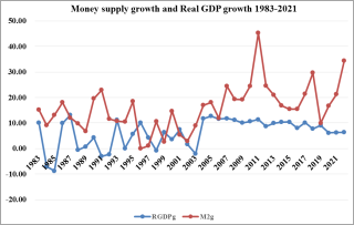
. Real GDP growth has been fluctuating in rate. The growth pattern has somewhat altered, as seen below, entering double-digit growth from 2003/04.
The economy has received an extensive infusion of money for several reasons, including the expansion of government and private investment. Furthermore, spending on consumption rises in parallel with investment and employment growth. The countries' money growth fluctuated somewhat between 1982/83 to 2003/04; from 2003/04 to 2010/11, the money growth increased at a decreasing rate; from 2009/10 to 2010/11, the money growth increased significantly; and from 2010/11 to 2015/16, the money growth declined significantly. In the end, between 2016/17 to 2020/21, there were fluctuations in the money supply growth.
Figure 1. Money supply and Real GDP growth.
Both of the methods that a rise in money supply encourages investment and expenditure by lowering interest rates and giving consumers more money, which makes them experience greater and encourages spending. Businesses increase output and make more raw material purchases in response to increased sales. The expansion of company activity drives up both the demand for capital goods and labor. The monetarist theory, which emphasizes that the money supply is a crucial macroeconomic factor that affects a country's economic growth, was developed by
| [27] | Friedman, B. M. (1986). Money, credit, and interest rates in the business cycle. In The American business cycle: Continuity and change (pp. 395-458). University of Chicago Press. |
[27]
. On the other hand, if the money supply expands faster than the economy, inflation may result. As a result, even when consumers have more money (or better access to money), their prices will still rise along with wages and input costs.
4.1.2. Domestic Credit and Economic Growth
Domestic credit, also known as domestic debt, refers to the total amount of money that is borrowed by individuals, businesses, and the government within a country. It is an important aspect of a country's financial system and plays a crucial role in driving economic growth.
Domestic credit plays a significant role in promoting economic growth by providing the necessary funds for investment, consumption, and development.
One of the main ways in which domestic credit contributes to economic growth is by providing the necessary capital for businesses to expand their operations. Domestic credit provides these businesses with the necessary funds to do so, thereby creating job opportunities and increasing production. This, in turn, leads to an increase in GDP and overall economic growth.
To investigate the relationship between domestic credit and economic growth, several studies have been conducted to explore the impact of domestic credit on economic development. Murari, K.
| [46] | Murari, K. (2017). Financial development–economic growth nexus: Evidence from South Asian middle-income countries. Global Business Review, 18(4), 924-935. |
[46]
indicated a significant association between domestic credit provided by the banking sector and economic growth, emphasizing the importance of credit allocation and financial regulation for economic development. Similarly,
| [20] | Dinh, D. V. (2020). Forecasting domestic credit growth based on ARIMA model: Evidence from Vietnam and China. Management Science Letters, 10(5), 1001-1010. |
[20]
emphasized the impact of domestic credit growth on GDP, providing insights for policymakers to understand the relationship between domestic credit and economic growth.
However, it is essential to note that excessive domestic credit can also have adverse effects on economic growth. If not managed properly, it can lead to inflation, which decreases the purchasing power of consumers and can hinder economic growth. Therefore, governments must strike a balance between providing enough credit to stimulate economic growth and avoiding excessive credit that can lead to inflation. Ozili, P. K., et. al found that abnormal increases in domestic credit to the private sector have a significant negative effect on real GDP growth
| [63] | Ozili, P. K., Oladipo, O., & Iorember, P. T. (2023). Effect of abnormal increase in credit supply on economic growth in Nigeria. African Journal of Economic and Management Studies. |
[63]
, particularly during crisis years. Similarly,
| [21] | Ductor, L., & Grechyna, D. (2018). Financial development, real sector output, and economic growth. International Review of Economics and Finance, 393-405. |
[21]
highlighted that rapid growth in private credit, without a corresponding increase in real output, leads to a negative effect of financial development on economic growth.
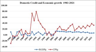
Figure 2. Domestic Credit and Economic growth.
Accordingly, in Ethiopia financial reform has been made during ERDF regime in Ethiopia in order to satisfy ever increasing demand for credit by private sector. The growth of domestic credit is fluctuating since 1982/83 to 1992/93 and highly increases 1991/92 to 1992/93 but largely decrease 1994/95 to 1999/00. Hence, as indicate below the growth of domestic credit is quiet similar to that of money supply.
4.1.3. Interest Rate and Economic Growth
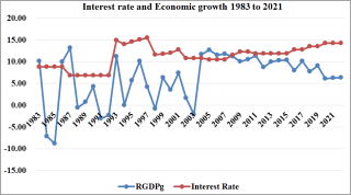
Interest rate is one of the most important tools used by central banks to regulate the economy. It is the rate at which banks can borrow money from the central bank or other financial institutions. The interest rate has a direct impact on economic growth, as it affects the cost of borrowing for businesses and individuals. The main goal of central banks is to maintain price stability and promote economic growth. They use interest rates as a tool to achieve these objectives. When the economy is growing too quickly, central banks may increase interest rates to slow down the pace of economic growth. On the other hand, when the economy is in a recession or facing slow growth, central banks may decrease interest rates to stimulate economic growth. When interest rates are low, businesses can borrow at a lower cost, which encourages them to invest in new projects and expand their operations. Another way in which interest rates impact economic growth is through its effect on inflation. When interest rates are low, it can lead to an increase in inflation as businesses and consumers are more likely to borrow and spend. Interest rates also play a crucial role in controlling the exchange rate of a country's currency. When interest rates are high, it can make the currency more attractive to foreign investors, leading to an increase in demand for the currency.
| [47] | Maiti, M., Esson, I. A., & Vuković, D. (2020). The impact of interest rate on the demand for credit in Ghana. Journal of Public Affairs, 20(3), e2098. |
[47]
Studied the impact of interest rates on the demand for credit in Ghana and highlighted the importance of real interest rates in inducing economic growth.
| [5] | Ali, M. A., Saifullah, M. K., & Kari, F. B. (2015). The impact of key macroeconomic factors on economic growth of Bangladesh: a VAR Co-integration analysis. International Journal of Management Excellence, 6(1), 667-673. |
[5]
On Bangladesh found that real interest rates have an impact on economic growth in the long run, further supporting the negative relationship between interest rates and economic growth.
Figure 3. Interest rate and Economic growth.
4.1.4. Trade Openness and Economic Growth
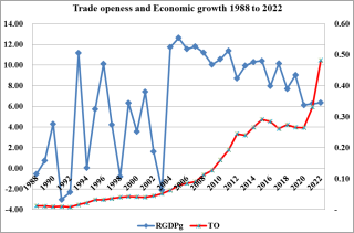
Trade openness refers to the degree to which a country engages in international trade and opens up its economy to foreign goods, services, and investments. Economic growth, on the other hand, refers to the increase in a country's production of goods and services over some time. Both trade openness and economic growth are crucial factors in determining a country's economic development and are closely interlinked.
Figure 4. Trade openness and Economic growth.
When a country opens up its economy to trade, it allows for the free flow of goods, services, and investments across its borders. This leads to increased competition among domestic producers, as they now have to compete with foreign firms. This competition drives innovation and efficiency, as domestic firms strive to produce better quality goods at lower prices to remain competitive. This, in turn, leads to increased productivity and economic growth. This leads to an increase in the purchasing power of consumers, which in turn boosts economic growth. However, trade openness can also have some negative effects on economic growth. One of the major concerns is that it can lead to job losses in certain industries that cannot compete with cheaper imports. This can have a negative impact on the economy, as it can lead to unemployment and a decrease in domestic production.
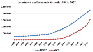
4.1.5. Investment and Economic Growth
Investment and economic growth are closely intertwined and have a significant impact on each other. Investment refers to the allocation of resources, such as money, time, and effort, towards a project or business venture with the expectation of future profits. Both investment and economic growth play a crucial role in the development of a country and have a positive effect on the overall well-being of its citizens. Firstly, investment is a key driver of economic growth. When businesses and individuals invest in new projects or expand their existing ones, it leads to an increase in production and employment opportunities. This, in turn, leads to a rise in consumer spending and boosts economic growth. Moreover, investment also leads to technological advancements and innovation, which are crucial for economic growth. When businesses invest in research and development, they come up with new and improved products and services that cater to the changing needs and demands of consumers. This not only contributes to economic growth but also helps in creating a competitive market environment, leading to more choices and better quality products for consumers. As shown below graph there is positive relationship between Investment and Real GDP. This means investment and real GDP move in the same direction. As investment increased, Real GDP also increased. And when investment decreased, Real GDP also decreased.
Figure 5. Investment and economic growth.
Furthermore, investment also has a positive impact on the overall standard of living in a country. When there is economic growth, there is an increase in the income of individuals, which leads to an improvement in their standard of living.
4.2. Econometric Results
4.2.1. Unit Root Test
Unit root test, also known as stationarity test, is a statistical method used to determine the presence of a unit root in a time series data. It is an important tool in time series analysis as it helps to identify whether a variable follows a stationary or non-stationary process. Stationarity refers to the statistical properties of a time series that remain constant over time, such as mean and variance. Before analyzing the estimated results for the VECM model to co-integration, the unit root tests are used to assess the order of integration of the variables. First, Empirical analysis by testing the unit roots in RGDP, M
2, GCF, CPS, CPI, REER, TO and RLR is used in this stage by applying the Augmented Dickey fuller (ADF) test. Therefore, to confirm that the data are stationary and stable, so the (ADF) test to test the null of unit root against the alternative of stationary has been conducted. The ADF test results presented for all variables with trend and intercept as in
table 1.
Table 1. Unit root test result.
Variables | With Intercept | With Intercept and trend |
t-statistic | t-statistic |
Level | 1st difference | Level | 1st difference |
LRGDP | 2.174 | -4.174* | -2.660 | -5.514* |
LM2 | 2.070 | -3.081* | -0.107 | -3.939* |
LCPS | -0.011 | -3.047* | -3.753 | -3.703* |
LGCF | 1.341 | -5.616* | -2.176 | -5.976* |
LREER | -2.068 | -5.357* | -1.986 | -5.222* |
LTO | -0.172 | -5.744* | -3.719 | -5.649* |
RLR | -2.235 | -7.832* | -4.027 | -7.705* |
LCPI | 2.122 | -4.759* | -0.385 | -3.940* |
Source: Source: Author’s Computation of E-Views 12 Results Note: * indicates significance at 5%. The test is applied to first differences of all variables stationary with constant and with constant and trend, hence the variables are considered as I(1) process. One of the main conditions for using VECM model when all variables are stationary at first difference.
4.2.2. Lag Length Selection
The choice of lag length can have a significant impact on the results and conclusions drawn from a time series analysis. Therefore, it is crucial to carefully select the appropriate lag length for a given dataset. Before delving into the criteria for selecting the lag length, let us first understand what a lag length is. In time series analysis, lag length refers to the number of past observations used to predict the current value of a variable. It is an essential parameter in various time series models, such as Autoregressive (AR), Moving Average (MA), and Autoregressive Moving Average (ARMA) models.
Table 2. VAR Lag Order Selection Criteria.
Lag | LogL | LR | FPE | AIC | SC | HQ |
0 | -94.49575 | NA | 4.83e-08 | 5.856900 | 6.212408 | 5.979621 |
1 | 273.5045 | 546.7432 | 1.52e-15 | -11.51454 | -8.314970* | -10.41005 |
2 | 368.9121 | 98.13358* | 4.69e-16* | -13.30927* | -7.265628 | -11.22300* |
LR: sequential modified LR test statistic (each test at 5% level)
FPE: Final prediction error
AIC: Akaike information criterion
SC: Schwarz information criterion
HQ: Hannan-Quinn information criterion
Table 2. Reveals that while LR, FPE, AIC and HQ information criteria chooses 2 lag orders, SC selects 1 lag order for the VAR. Therefore, the information criteria provide the conflicting 2 lag order VAR applied. Thus, the Johansen co-integration test conducted under the assumption of no trend but a constant in the series and 1 lag intervals.
4.2.3. Johansen Co-Integration Test
The Johansen co-integration test is a statistical method used to determine the long-run relationship between two or more stationary time series variables. The concept of co-integration was first introduced by
| [26] | Engle, R. F., & Granger, C. W. (1987). Co-integration and error correction: representation, estimation, and testing. Econometrica: journal of the Econometric Society, 251-276. |
[26]
. The co-integration test is based on the idea that if two or more variables are co-integrated, then there must be a long-term equilibrium relationship between them. This means that any deviation from this equilibrium will eventually be corrected, and the variables will return to their long-term relationship. In other words, the co-integration test helps in identifying whether two or more variables are bound together in the long run, even though they may show short-term deviations. The Johansen co-integration test is an extension of the Engle-Granger co-integration test, which only allows for the analysis of two variables. The Johansen test, on the other hand, can handle multiple variables and allows for the estimation of the number of co-integrating relationships between them. This makes it a more powerful and flexible tool for analyzing time series data. The results in
Table 3 reveal that both the 𝜆𝑡𝑟𝑎𝑐𝑒 and 𝜆𝑚𝑎𝑥 statistics rejected the null hypothesis of no co-integration against the alternative, as evidenced by test statistics, which are greater than the critical values. This suggests that there exists long-run relationship among variables. In addition, Johansen test reveals that there is more than one co-integrating relationships. Specifically, Trace test indicates 5 cointegrating eqn(s) at the 0.05 level and Max-eigenvalue test indicates 3 cointegrating eqn(s) at the 0.05 level.
Table 3. Co-integration Rank test.
Hypothesized (No. of CE(s) | Trace | Critical Value | Prob.** | Max-Eigen | Critical Value | Prob.** |
None | 276.243 | 159.53 | 0.000* | 79.901 | 52.363 | 0.000* |
At most 1 | 196.342 | 125.615 | 0.000* | 66.391 | 46.231 | 0.000* |
At most 2 | 129.951 | 95.754 | 0.000* | 39.905 | 40.078 | 0.052 |
At most 3 | 90.045 | 69.819 | 0.001* | 34.765 | 33.877 | 0.039* |
At most 4 | 55.280 | 47.856 | 0.009* | 25.95 | 27.584 | 0.080 |
At most 5 | 29.33 | 29.797 | 0.057 | 16.602 | 21.132 | 0.192 |
At most 6 | 12.728 | 15.495 | 0.125 | 10.291 | 14.265 | 0.194 |
At most 7 | 2.437 | 3.841 | 0.119 | 2.437 | 3.841 | 0.119 |
4.2.4. Model Stability and Diagnostic Test
Diagnostic tests are an essential tool in econometrics that helps in evaluating the validity and reliability of a statistical model. They are used to identify any potential issues or problems with the model and provide a measure of its overall fit. One of the most common diagnostic tests used in econometrics is the residual test.
There are several types of residual tests used in econometrics, and each serves a specific purpose. The most widely used ones are the normality test, heteroscedasticity test, and autocorrelation test.
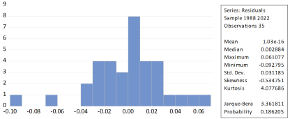
The normality test examines whether the residuals follow a normal distribution, which is a fundamental assumption in many econometric models. Non-normality may indicate that the model is not capturing all the factors affecting the data, leading to biased estimates. This test is typically done by plotting the residuals on a histogram or a normal probability plot, and any significant deviations from a straight line suggest non-normality.
Figure 6. Normality test.
Heteroscedasticity, which means unequal variance, is another issue that can affect the validity of an econometric model. It occurs when the residuals have different variances across the range of data. This can lead to biased standard errors and confidence intervals, making the model less reliable. The most commonly used test for heteroscedasticity is the Breusch-Pagan test, which compares the variance of the residuals with the independent variables. A significant result indicates heteroscedasticity, and corrective measures such as using robust standard errors can be applied.
Table 4. Heteroskedasticity test.
Heteroskedasticity Test: Breusch-Pagan-Godfrey |
Null hypothesis: Homoskedasticity |
F-statistic | 0.8440 | Prob. F(16,18) | 0.6306 |
Obs*R-squared | 15.0028 | Prob. Chi-Square (16) | 0.5244 |
Scaled explained SS | 11.7791 | Prob. Chi-Square (16) | 0.759 |
Autocorrelation, also known as serial correlation, is a phenomenon where the error terms in a model are correlated with each other. This can happen when the data is collected over time, and the observations within a time series are not independent. Autocorrelated residuals can lead to biased coefficient estimates and unreliable hypothesis testing.
Table 5. Serial correlation test.
Breusch-Godfrey Serial Correlation LM Test: |
Null hypothesis: No serial correlation at up to 2 lags |
F-statistic | 0.472 | Prob. F(2,23) | 0.630 |
Obs*R-squared | 1.381 | Prob. Chi-Square(2) | 0.501 |
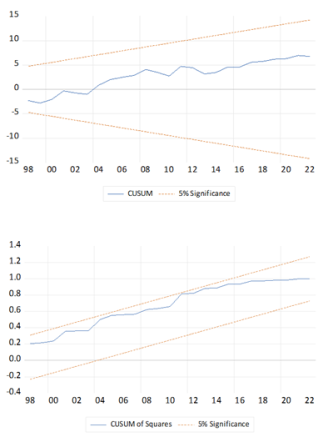
Figure 7. CUSUM test and CUSUM of square test Stability.
Tests of Autocorrelation, Normality and Hetroskedasticity test of the VECM Models are conducted with the help Lagrange-multiplier, Jarque-Bera test and white tests. This test is used to confirm the basic assumptions regarding the residual and validity of the results in the study. From the tests, it was found that the nulls of no serial correlation, normality and homoskedasticity in the residuals couldn’t be rejected in all cases.
4.2.5. Test for Vector Error Correction Model
Vector Autoregressive Models, or VARs, are specifically applied in Vector Error Correction Mechanism (VECM) models. Error correction terms are introduced into the VAR models in order to specify VECM models. If the system's variables are co-integrated, or have a long-run relationship, the VECM approach is applied.
By separating the variables and introducing error correction terms, any VAR model may be expressed as VECM. VECM, however, is only applied in the context of cointegrating or long-term relationships. The VAR model needs to be used if there is no cointegration or if the variables are stationary.
(i). The Estimation of Long-Run Model
The relevance of the long-run variables is taken into consideration while identifying the variables that collectively form the cointegrating vectors.
Table 6. Co-integrating (𝛽) Coefficients.
Variables | Coefficients | Standard error | t-statistics |
LRGDP(-1) | 1.000 | . | . |
LREER(-1) | -0.105 | 0.042 | -2.512* |
LM2(-1) | -0.384 | 0.043 | -8.987* |
LGCF(-1) | -0.306 | 0.023 | -13.375* |
LCPS(-1) | -0.049 | 0.017 | -2.903* |
LCPI(-1) | 0.534 | 0.055 | 9.782* |
LTO(-1) | -0.055 | 0.027 | -2.046* |
RLR(-1) | 0.037 | 0.004 | 10.516* |
C | -6.981 | . | . |
LRGDP=0.105LREER+0.384LM2+0.306LGCF+0.049LCPS-0.534LCPI+0.055LTO-0.037RLR+6.981
The coefficients' signs correspond with theoretical expectations, as previously mentioned. The coefficients of the consumer price index, trade of openness, real lending rate, gross capital formation (investment), real effective exchange rate, broad money supply, and private sector for credit are significant at the five percent level, according to the t-test statistics.
The coefficient on real effective exchange rate for the real exchange rate is positive and significant. This result indicate that if all other explanatory variables are held constant, as REER increases by 1percent, economic growth increase by 0.105 long run. As foreign currency (the value of the dollar) increases, economic growth increases. The real effective exchange rate has a significant impact on economic growth in Ethiopia. The country's heavy reliance on international trade makes it vulnerable to fluctuations in the REER, which can affect its trade balance, foreign investment, and macroeconomic stability. The government's recent policies to increase the REER have shown positive results, with a decrease in the trade deficit and an increase in foreign investment. However, continuous monitoring and management of the REER are necessary to ensure sustained economic growth in Ethiopia.
| [68] | Rao, P. N., & Tolcha, T. D. (2016). Determinants of real exchange rate in Ethiopia. International Journal of Research-GRANTHAALAYAH, 4(6), 183-210. |
[68]
Which shows that REER increase’s in the time of higher export capacity and influences the rate of domestic private investments positively. Having a weaker currency relative to the rest of the world can help boost exports.
| [22] | Di Nino, V., Eichengreen, B., & Sbracia, M. (2011). Real exchange rates, trade, and growth: Italy 1861-2011. Bank of Italy Economic History Working Paper, (10). |
[22]
Studied the effect of exchange rate on economic growth for Italy during the period 1861-2011. They have shown that the undervaluation promotes growth by increasing exports, especially productivity. A theoretical analysis by
| [69] | Razmi, A., Rapetti, M., & Skott, P. (2012). The real exchange rate and economic development. Structural change and economic dynamics, 23(2), 151-169. |
[69]
showed that the real undervaluation positively affects economic growth for two reasons. On the one hand, it shifts domestic consumption towards non-tradable goods. On the other hand, it increases profitability and investment in the tradable goods sector.
| [33] | Glüzmann, P. A., Levy-Yeyati, E., & Sturzenegger, F. (2012). Exchange rate undervaluation and economic growth: Díaz Alejandro (1965) revisited. Economics Letters, 117(3), 666-672. |
[33]
Have shown that the depreciation of the national currency makes it possible to increase savings and investment, which positively affects economic growth.
| [8] | Aman, Q., Ullah, I., Khan, M. I., & Khan, S. U. D. (2017). Linkages between exchange rate and economic growth in Pakistan (an econometric approach). European Journal of Law and Economics, 44, 157-164. |
[8]
Studied the link between exchange rate and economic growth for Pakistan. Using data covering the period 1976 - 2010 and the least-squares technique, the authors have shown that a depreciation of the national currency positively affects economic growth since depreciation encourages exports and imports of substitution.
The long run model in
table 6. Shows that broad money supply (M
2) has a significant positive effect on the economic growth.
That is, a one percent increases in money supply
results in about 0.38% increase in economic growth
in the long run. This finding is in line with the findings by
| [74] | Tabi, H. N., & Ondoa, H. A. (2011). Inflation, money and economic growth in Cameroon. International Journal of financial research, 2(1), 45-56. |
[74]
, who reported significant positive effect of money supply on economic growth in their study in Cameroon.
| [16] | Chude, N. P., & Chude, D. I. (2016). Impact of broad money supply on Nigerian economic growth. IIARD International Journal of Banking and Finance Research, 2(1), 46-52. |
[16]
We found that the money supply and economic growth in Nigeria are positively and significantly related. This suggests that M
2 dominates the relationship between prices and output.
| [34] | Galadima, M. D., & Ngada, M. H. (2017). Impact of money supply on economic growth in Nigeria (1981–2015). Dutse Journal of economics and development studies, 3(1), 133-144. |
[34]
The findings reveal that there is statistically significant positive relationship between money supply and economic growth both in short run and long run.
| [64] | Onyeiwu, C. (2012). Monetary policy and economic growth of Nigeria. Journal of Economics and Sustainable development, 3(7), 62-70. |
[64]
The result of the analysis shows that monetary policy presented by money supply exerts a positive impact on GDP growth.
Impact on GDP growth a Money supply also has a direct impact on employment. An increase in money supply leads to higher investment, which, in turn, creates more job opportunities. This can have a positive effect on economic growth as it increases consumer spending and boosts overall economic activity. An increase in money supply can also lead to lower interest rates. This is because banks have more money to lend, and competition among them increases, leading to a decrease in interest rates. Lower interest rates make it easier for businesses and individuals to borrow money, which can stimulate economic growth. When there is an increase in money supply, businesses tend to expand their operations, leading to an increase in employment opportunities. This, in turn, leads to an increase in consumer spending, which further boosts economic growth.
The coefficient on GCF (Investment) found for the real GDP is positive and significant. A one percent increases in the investment 0.31 percent change in real GDP under the study period. It indicates that one of the most significant impacts of investment on economic growth is the creation of jobs. When individuals or businesses invest in a particular sector, it leads to the creation of new enterprises, expansion of existing ones, and the development of new industries. All of these activities require a workforce, thus generating employment opportunities for people. This, in turn, leads to an increase in income levels, which boosts consumer spending and ultimately drives economic growth. Investment also has a direct impact on productivity. When companies invest in new technologies, machinery, and equipment, it leads to increased efficiency and productivity. This, in turn, leads to higher output and lower costs, making companies more competitive in the market. As a result, businesses can expand, leading to higher economic growth. Additionally, investment in research and development also drives innovation, which further boosts productivity and economic growth. However, it is essential to note that the effects of investment on economic growth are not immediate. It takes time for investments to yield results and contribute to economic growth. Investments are critical to economic growth that will lead to rapid economic development and reduce poverty
| [53] | Nnanna, J. (2004). Financial sector development and economic growth in Nigeria: An empirical investigation. Economic and Financial Review, 42(3), 2. |
[53]
.
The coefficient on Trade Openness found for the real GDP is positive and significant. It indicates that one of the most significant effects of trade openness on economic growth is its impact on productivity. When countries open up their borders and remove trade barriers, it allows for the free flow of goods and services, which leads to increased competition. This competition, in turn, forces firms to become more productive and efficient to remain competitive. As a result, there is an increase in the overall productivity of the economy, leading to economic growth. Another effect of trade openness on economic growth is its impact on innovation and technology transfer. When countries engage in trade, they are exposed to new ideas, technologies, and practices from other countries. This exposure can lead to innovation and the adoption of new technologies, which can enhance productivity and economic growth. For instance, China's rapid economic growth in recent decades can be attributed, in part, to its openness to trade, which has led to the transfer of technology from other countries. According to our study a 1 percent increase in trade openness can lead to a 0.05% increase in productivity, which can have a significant impact on economic growth. Confirm the result by
| [48] | Malefane, M. R. (2018). Trade openness and economic growth: experience from three SACU countries. Published doctoral dissertation. University of South Africa, Pretoria. |
[48]
According to the long-run empirical results obtained, it was found out that trade openness has a positive and significant impact on economic growth. Das, A. and Paul, B. P. found that trade openness has a positive effect on economic growth in Asia
| [23] | Das, A., & Paul, B. P. (2011). Openness and growth in emerging Asian economies: Evidence from GMM estimations of a dynamic panel. Economics Bulletin, 31(3), 2219-2228. |
[23]
.
The coefficient on credit for private sector found for the real GDP is positive and significant. It suggests that Credit is an essential tool for businesses to invest in new projects, expand their operations, and innovate. It allows businesses to take advantage of new opportunities and increase their productivity, which ultimately leads to economic growth. With the availability of credit, businesses can purchase new equipment, hire more employees, and develop new products and services. The private sector credit coefficient (CPS) is 0.049. This suggests that throughout the study period, a one percent change in credit to the private sector brought about a 0.049 percent change in real GDP, holding other factors constant. This conclusion is in line with the findings of a research conducted in Ethiopia by
| [35] | Genemo, A. G. (2022). The impact of private sector credit on economic growth in Ethiopia (Doctoral dissertation, HU). |
[35]
.
The coefficient on Consumer price index (inflation) found for the economic growth is negative and significant. It suggests that inflation can have a significant impact on economic growth. It can decrease purchasing power, discourage investment, increase interest rates, decrease exports, and affect income distribution. One percent increase in Consumer price index (inflation) will decrease economic growth by 0.53 percent. This is consistent with finding of
| [9] | Ahmed, S., & Mortaza, G. (2005). Inflation and economic growth in Bangladesh. Policy Analysis Unit Working Paper Series: WP, 604. |
[9]
found a statistically significant long-run negative relationship between inflation and economic growth.
| [75] | Tien, N. H. (2021). Relationship between inflation and economic growth in Vietnam. Turkish Journal of Computer and Mathematics Education (TURCOMAT), 12(14), 5134-5139. |
[75]
The results confirm the existence of the threshold at 6 per cent inflation point, and the negative impacts on GDP growth of hyperinflation above the threshold and too low inflation beyond the threshold.
In this study, Real lending rate (RLR) has a negative and significant effect at 5% level of significance on real GDP in long run. This means keeping other things constant, a one percent increases in RLR results 0.037 decrease the economic growth (real GDP) in the long run. It implies that a high level of lending interest rates raises the businesses and individuals are less likely to borrow money. This leads to a decrease in economic activity, as businesses scale back their operations, and individuals delay large purchases. The decrease in economic activity can lead to a decrease in job creation and consumer spending, resulting in a slowdown in economic growth. However, interest rates are high; borrowing becomes more expensive, leading to a decrease in demand and a decrease in the prices of goods and services, resulting in lower inflation. This is consistent with finding of
| [49] | Mutinda, D. M. (2014). The effect of lending interest rate on economic growth in Kenya (Doctoral dissertation, University of Nairobi). |
[49]
the study established that there is a negative relationship between interest rate and the economic growth. Daniel, Berko, et. al investigated the effect of interest rate spread on Ghanaian economic growth using annual time series data from 1975 to 2018
| [24] | Daniel, Berko, Paul Hammond, and Edmond Amissah. "The effect of interest rate spread on economic growth: Ghana’s perspective." International Journal of Business and Management Review 10, no. 2(2022): 1-23. |
[24]
. The study used the Engel-Granger two-step procedure which uses the OLS technique to establish both the long-run and short-run relationships between interest rate spread and economic growth. The study found that interest rate spread is a statistically important determinant of economic growth in Ghana but has a negative impact in the long run.
(ii). Estimation of the Error-Correction Model
Having already obtained the long-run model and estimated the coefficients, the next step will be estimation of coefficients of the short-run dynamics that have important policy implications. Hence, an error correction model will be estimated which incorporates the short term interactions and the speeds of adjustment towards long run model.
Table 7. Short-Run coefficients.
Variables | Coefficients | Standard Error | t-value |
D(LRGDP(-1)) | 0.018 | 0.194 | 0.092 |
D(LTO(-1)) | 0.048 | -0.064 | 0.748 |
D(LREER(-1)) | -0.019 | -0.083 | -0.226 |
D(LM2(-1)) | 0.093 | -0.122 | 0.761 |
D(LGCF(-1)) | -0.111 | -0.079 | -1.410 |
D(LCPS(-1)) | 0.166 | -0.098 | 1.687 |
D(LCPI(-1)) | -1.073 | -0.526 | -2.040 |
D(RLR(-1)) | 0.002 | -0.001 | 3.082 |
ECT(-1) | -0.316 | -0.146 | -2.165 |
C | 0.125 | -0.052 | 2.417 |
R-squared | 0.5218 | Sum sq. resides. | 0.0331 |
Adj. R-squared | 0.3497 | F-statistic | 3.0312 |
Denotes significance at 5 percent level
In the above table shows that the coefficient of the error correction term is significant with expected sign and reasonable magnitude (ECM =-0.316). The coefficient of the error correction term of the real GDP is negative and less than one. This result ensures that real GDP (economic growth) convergences to its long run equilibrium. The coefficient of the error term (ECT(-1)) implies that the deviation from long run equilibrium level of real GDP in the current period is corrected by 31.6% in the next period to bring back equilibrium when there is a shock to a steady state relationship.
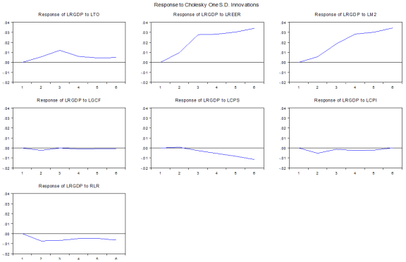
(iii). Impulse Response Analysis
Impulse response analysis reveals a wealth of information on dynamic effects that is missing in both static studies and those dynamic studies that do not employ these techniques.
Figure 8. Presents the results from the impulse response analysis performed on the VECM regression. In this figure since the study focuses on the effects of the economic growth, only the responses of the economic growth to shocks in its effects are presented. These impulse response functions show the dynamic response of the economic growth to a one-period standard deviation shock to the innovations of the system. Additionally, they indicate the directions and persistence of the response to each of the shocks for ten years.
Figure 8. Impulse Response Analysis.
For the most part, the impulse response functions have the expected pattern and confirm the results from the short run relationship analysis. A one period standard deviation positive shock to LCPS the real GDP by decrease 0.002 percent and it also permanent shock or are not converge to zero. A one period standard deviation shock to LGCF (investment) the real GDP by decrease 0.004 percent and the effects of shock converge to zero after some period. A one period standard deviation shock to RLR the real GDP by decrease 0.002 percent, it also permanent shock or are not converge to zero. A one period standard deviation shocks to LTO the real GDP by increase 0.008 percent, but it is also transitory shock or converges to zero after 3 years. A one period standard deviation shocks to LM2 the real GDP by increase 0.024 percent and it also permanent shock or are not converge to zero. A one period standard deviation shocks to LREER the real GDP by increase 0.010 percent and it also permanent shock. A one period standard deviation shocks to LCPI the real GDP by decrease 0.002 percent, but also gradually levels off in about 6 years or converges to zero.
(iv). Variance Decomposition Analysis
Variance decomposition analysis provides a way of determining the relative importance of shocks to each of the transmission of monetary policy channel and economic growth in explaining variations in the economic growth. The following table shows the proportion of the forecast error variance in the economic growth.
Table 8. Variance decomposition of the real GDP.
Period | S.E. | LRGDP | LREER | LM2 | LGCF | LCPS | LCPI | LTO | RLR |
1 | 0.036 | 100 | 0.000 | 0.000 | 0.000 | 0.000 | 0.000 | 0.000 | 0.000 |
2 | 0.063 | 93.975 | 0.843 | 1.259 | 0.174 | 0.410 | 0.098 | 1.921 | 1.320 |
3 | 0.091 | 81.251 | 4.470 | 6.696 | 1.592 | 0.445 | 0.413 | 3.934 | 1.200 |
4 | 0.116 | 76.106 | 6.211 | 11.225 | 1.296 | 0.272 | 0.309 | 3.672 | 0.909 |
Cholesky Ordering: LRGDP LREER LM2 LGCF LCPS LCPI LTO RLR |
The above table reports only the variance decomposition in the real GDP and analysis the relative importance of each of its explanatory variables in influencing its movements, because the interest is to know the movements of the real GDP following shocks to itself or its explanatory variables. In the first period all of the variance in the real GDP is explained by its own shocks. For the second period a head forecast error variance the real GDP itself explains about 94 percent of its variation, while all its explanatory variables explain only the remaining 6 percent. Out of this 6 percent the real effective exchange rate explain about 0.843 percent, money supply explain about 1.259 percent, gross capital formation explain about 0.174 percent, credit for private sector explain about 0.410 percent, consumer price index(inflation) explain about 0.098 percent, trade openness explain about 1.921 percent and real lending rate explain about 1.32 percent. In the third period the real GDP explains about 81 percent of its own variation, while its explanatory variables explain the remaining 19 percent. Out of this 19 percent the real effective exchange rate explain about 4.47 percent, money supply explain about 6.696 percent, gross capital formation(investment) explain about 1.592 percent, credit for private sector explain about 0.445 percent, consumer price index(inflation) explain about 0.413 percent, trade openness explain about 3.934 percent and real lending rate 1.32 percent In the fourth period the real GDP explains about 76 percent of its own variation, while its explanatory variables explain the remaining 24 percent. Out of this 24 percent the real effective exchange rate explain about 6.2 percent, money supply explain about 11.23 percent, gross capital formation(investment) explain about 1.3 percent, credit for private sector explain about 0.272 percent, consumer price index(inflation) explain about 0.31 percent, trade openness explain about 3.7 percent and real lending rate 1 percent.
(v). Causality Approach Analysis
Granger causality only provides information about forecasting ability; it does not provide insight into the true causal relationship between two variables.
The finding of stationarity of the variables and co integration between economic growth (real gross domestic product) and monetary policy implies that there is long-run causality in at least one direction
| [26] | Engle, R. F., & Granger, C. W. (1987). Co-integration and error correction: representation, estimation, and testing. Econometrica: journal of the Econometric Society, 251-276. |
[26]
. Therefore, it would be useful to test long-run causality if co integration is found. The result of the long run causality between the dependent variable real domestic product and the macroeconomic variable is given in table below.
Table 9. Pairwise Granger Causality Tests.
Null Hypothesis: | Obs | F-Statistic | Prob. |
LREER does not Granger Cause LRGDP | 36 | 1.218 | 0.278 |
LRGDP does not Granger Cause LREER | 0.048 | 0.828 |
LM2 does not Granger Cause LRGDP | 36 | 0.558 | 0.460 |
LRGDP does not Granger Cause LM2 | 6.175 | 0.018* |
LGCF does not Granger Cause LRGDP | 36 | 2.729 | 0.108 |
LRGDP does not Granger Cause LGCF | 1.840 | 0.184 |
LCPS does not Granger Cause LRGDP | 36 | 1.061 | 0.311 |
LRGDP does not Granger Cause LCPS | 0.843 | 0.365 |
LCPI does not Granger Cause LRGDP | 36 | 0.018 | 0.895 |
LRGDP does not Granger Cause LCPI | 5.956 | 0.020* |
LTO does not Granger Cause LRGDP | 36 | 8.297 | 0.007* |
LRGDP does not Granger Cause LTO | 0.041 | 0.842 |
RLR does not Granger Cause LRGDP | 36 | 0.003 | 0.957 |
LRGDP does not Granger Cause RLR | 2.100 | 0.157 |
“*” represents the level of significance at 5% respectively
Source: Own Compilations of Eviews-12 result
The estimation result of VECM model the above
table 9 result of the Granger causality test from money supply(LM
2) to real gross domestic product (LRGDP) are not rejected based on the fact that the null hypothesis that varies in money supply(LM
2) does not Granger real gross domestic product (LRGDP), given the probability 0.46 which is insignificant but there are causality moving from real gross domestic product (LRGDP) to money supply(LM
2) by having 0.018 probability which is significant at 5% level of significance this case we can reject the null which states that real gross domestic product (LRGDP) not Granger Cause money supply(LM
2) the indication of this result is that there exist a unit-directional causality from money supply (LM
2) to real gross domestic product (LRGDP) of Ethiopia.
Based on the p-value corresponding to the F-statistic (0.007), we reject the null hypothesis that trade openness does not Granger cause real gross domestic product at 5% level of significance. However, the F-statistic and the associated p-vale (0.842) indicates that we do not reject the null hypothesis that real gross domestic product does not Granger cause trade openness at 5% level of significance. The Granger Causality test shows unidirectional causality between trade openness and real gross domestic product. Olufemi, S. M. found a unidirectional relationship between openness and growth
| [65] | Olufemi, S. M. (2004). Trade openness and economic growth in Nigeria: Further evidence on the causality issue. South African Journal of Economic and Management Sciences, 7(2), 299-315. |
[65]
. This indicates that an increasing level of openness will be beneficial, depending on the level of economic development in Nigeria. Nduka, E. K. reported a unidirectional causality ranging from economic growth to openness without a feedback in the pre-Structural Adjustment Programmed period (growth-led trade)
| [55] | Nduka, E. K. (2013). Openness and economic growth in Nigeria. Journal of Education and practice, 4(1), 68-73. |
[55]
.
Based on the p-value corresponding to the F-statistic (0.895), we do not reject the null hypothesis that Consumer price index (inflation) does not Granger cause real gross domestic product at 5% level of significance. However, the F-statistic and the associated p-vale (0.020) indicated a rejection of the null hypothesis that real gross domestic product does not Granger cause Consumer price index (inflation) at 5% level of significance. The Granger Causality test showed unidirectional causality between Consumer price index (inflation) and real gross domestic product. Erbaykal, E., and Okuyan, H. A. analyzed the relationship between inflation and economic growth for Turkey
| [25] | Erbaykal, E., & Okuyan, H. A. (2008). Does inflation depress economic growth? Evidence from Turkey. International Journal of Finance and Economics, 13(17). |
[25]
. They employed the co-integration and causality test, bounds test, and WALD test. They also found a uni-directional causal relationship flowing from inflation to economic growth.